CSC270 Sept 30 Lecture I: Numerical Analysis

Fundamental Theorem of Calculus


      b /
        | f(x) dx = F(b) - F(a)
      a /

where F(x) is the `antiderivative':

       d
      -- F(x) = f(x)
      dx

To compute integrals this way, we need to derive F(x) analytically.
For example, if f(x) = x^2, the antiderivative is 1/3 x^3.

Consider f(x) = sqrt( 1 + (cos x)^2 ).  This is the length of the
curve (x, sin x) for x in [0,pi].  There is no analytic expression for
the antiderivative of f(x)!

Thus, for some functions, we cannot use the fundamental theorem of
calculus and we must resort to numerical integration.



Numerical Integration

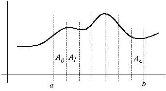
Recall that the definite integral

      b /
        | f(x) dx
      a /

is equal to the area under the curve f(x) in the interval [a,b].

We split the interval [a,b] into n smaller intervals, each of width
delta_x:

      a                          b
      |--------------------------|

      x0 x1 x2 x3 x4 x5 x6 x7 x8 x9
      |--|--|--|--|--|--|--|--|--|   nine intervals of width delta_x
         \  /                        Here, n = 9
          \/ width delta_x

Then 
      delta_x = (b-a) / n 
and
      x_i = a + i * delta_x

and the integral on [a,b] is just the sum over all the small intervals:

                          x_{i+1}
      b /           n-1   /
        | f(x) dx = sum(  |  f(x) dx  )
      a /           i=0   /
                          x_i

                    n-1
                  = sum( A_i )
                    i=0

where A_i is the area under the curve in the interval [ x_i, x_{i+1} ].



We will estimate A_i in each of the intervals and sum up the
estimates.  That will be our estimate of the integral.  Two things
affect the quality of our integral:

  - the interval size: smaller is better
  - the method of estimating A_i



Riemann Sums

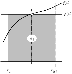
The first method of estimating A_i uses a constant function

  p(x) = c_i

to approximate f(x).  The constant function interpolates f(x) in the
middle of the interval.  Thus, c_i is chosen to be:

           x_i + x_{i+1}
  c_i = f( ------------- )
                 2

and the area under p(x) approximates the area A_i under f(x):


      
  A_i  ~  delta_x * c_i
       ~





Trapezoid Rule

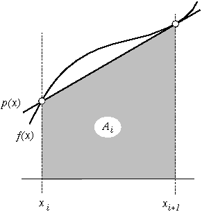
The second method of estimating A_i uses a linear function

  p(x) = b_i x + c_i

to approximate f(x) in the interval [ x_i, x_{i+1} ].  The
linear function interpolates f(x) at the endpoints of the
interval:

     p(x_i) = f(x_i)
and
     p(x_{i+1}) = f(x_{i+1})

and the area under p(x) approximates the area A_i under f(x):


                    f(x_i) + f(x_{i+1})
  A_i  ~  delta_x * -------------------
       ~                     2





Simpson's Rule

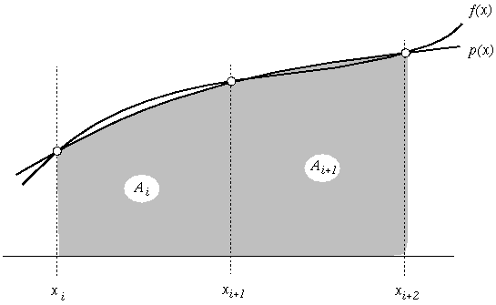
The third method of estimating A_i uses a quadratic function

  p(x) = a_i x^2 + b_i x + c_i

to approximate f(x) in the interval [ x_i, x_{i+1} ].  Here,
the quadratic function interpolates f(x) at three points:

     p(x_i) = f(x_i)
and
     p(x_{i+1}) = f(x_{i+1})
and
     p(x_{i+2}) = f(x_{i+2})

The area under p(x), which approximates A_i plus A_{i+1}, is

                              1
  A_i + A_{i+1} ~  delta_x * --- * ( f(x_i) + 4 f(x_{i+1}) + f(x_{i+2}) )
                ~             3





Summary

In each case, we split the interval [a,b] into many smaller intervals
of equal width.  We estimate the integral of f(x) on [a,b] with the
sum of our estimates for the areas A_i of the smaller intervals.

For example, if we use Simpson's rule and split the interval [a,b]
into n smaller intervals, each of size (b-a)/n, we get

      b /              n-1
        | f(x) dx  =   sum( A_i )
      a /              i=0

                       n/2
                   =   sum( A_{2k-2} + A_{2k-1} )
                       k=1

                       n/2
                   ~   sum( delta_x * (1/3) * ( f(x_{2k-2}) + 4 f(x_{2k-1}) + f(x_{2k}) ) )
                   ~   k=1

                       delta_x   n/2
                   =   -------   sum( f(x_{2k-2}) + 4 f(x_{2k-1}) + f(x_{2k}) )
                          3      k=1

                       delta_x               n/2                    n/2-1
                   =   -------  ( f(x_0) + 4 sum( f(x_{2k-1}) ) + 2  sum( f(x_{2k}) ) + f(x_n) )
                          3                  k=1                     k=1