|
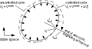
where [!]Uj are fixed control perturbations which are defined over a cycle and kij are fixed control perturbations which are defined over a cycle and kij are linear scaling are linear scaling
factors applied to [!]Uj.  Ki Ki is the vector of perturbation scaling factors and [!]U is a vector whose is the vector of perturbation scaling factors and [!]U is a vector whose
elements are the fixed control perturbations, [!]Uj, which remain the same from one cycle to the
next.  N N is the dimensionality of our control system and is equal to the number of state variables is the dimensionality of our control system and is equal to the number of state variables
which we wish to observe (and control).

Rather than using the complete system state, we choose to work with a small number of regulation
|

 1
2
3
4
5
6
7
8
9
10
11
12
13
14
15
16
17
18
19
20
21
22
23
24
25
26
27
28
29
30
31
32
33
34
35
36
37
38
39
40
41
42
43
44
45
46
47
48
49
50
51
52
53
54
55
56
57
58
59
60
61
62
63
64
65
66
67
68
69
70
71
72
73
74
75
76
77
78
79
80
81
82
83
84
85
86
87
88
89
90
91
92
93
94
95
96
97
98
99
100
101
102
103
104
105
106
107
108
109
110
111
112
113
114
115
116
117
118
119
120
121
122
123
124
125
126
127
128
129
130
131
132
133
134
135
1
2
3
4
5
6
7
8
9
10
11
12
13
14
15
16
17
18
19
20
21
22
23
24
25
26
27
28
29
30
31
32
33
34
35
36
37
38
39
40
41
42
43
44
45
46
47
48
49
50
51
52
53
54
55
56
57
58
59
60
61
62
63
64
65
66
67
68
69
70
71
72
73
74
75
76
77
78
79
80
81
82
83
84
85
86
87
88
89
90
91
92
93
94
95
96
97
98
99
100
101
102
103
104
105
106
107
108
109
110
111
112
113
114
115
116
117
118
119
120
121
122
123
124
125
126
127
128
129
130
131
132
133
134
135

