 |
 |
 |
 |
 |
 |
 |
 |
 |
 |
 |
 |
 |
 |
 |
 |
|
69
|
 |
|
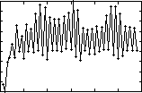
Two particular problems are apparent when viewing the generated motion:
- All three sampling strategies generate walks with step lengths which vary widely from
|

one step to the next as shown in Figure 4.12. This contrasts sharply with the uniform
step lengths generated when using up vector RVs.
|
 "Tightrope" walking, similar to that present in some up vector-based walks, is also "Tightrope" walking, similar to that present in some up vector-based walks, is also
|
 |
|
prevalent in the swing-COM trials.
|
The use of swing-COM RVs, however, makes a
|
 |
|
reasonable solution possible by choosing Qd with this problem in mind. with this problem in mind.
|
 |
|

0.5
0.4
0.3
0.2
0.1

 0 0 10 10 20 20 30 30 40 40 50 50 60 60
|
|
 |
|

|
|
 |
|
step
|
 |
|
Figure 4.12 - Step length vs step number, SP sampling,
 Qd Qd
 = [0.05,0] = [0.05,0]
|
 |
|

 0.3 0.3

 0.2 0.2

 0.1 0.1

 0 0

-0.1
-0.2

 0 0 10 10 20 20 30 30 40 40 50 50 60 60

 step step
|
|
 0.3 0.3

 0.2 0.2

 0.1 0.1

 0 0

-0.1
-0.2

 0 0 10 10 20 20 30 30 40 40 50 50 60 60
|
|
 |
|

|

|
|
 |
|
|
step
|
 |
|
(a) forward component
|
(b) lateral component
|
 |
|
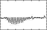
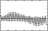
 Figure Figure  4.13 4.13 - Discrete RV values for SP sampling, - Discrete RV values for SP sampling,  Qd Qd = =  [0.0,±0.03]. [0.0,±0.03].
Compare with Figure 4.11. Larger lateral step-to-step variation means less tightrope walking.

The first problem will be addressed in the next chapter. To solve the second problem, the lateral
component of Qd
 is chosen to give the swing foot a displacement slightly away from the body and is chosen to give the swing foot a displacement slightly away from the body and
|
 |

 1
2
3
4
5
6
7
8
9
10
11
12
13
14
15
16
17
18
19
20
21
22
23
24
25
26
27
28
29
30
31
32
33
34
35
36
37
38
39
40
41
42
43
44
45
46
47
48
49
50
51
52
53
54
55
56
57
58
59
60
61
62
63
64
65
66
67
68
69
70
71
72
73
74
75
76
77
78
79
80
81
82
83
84
85
86
87
88
89
90
91
92
93
94
95
96
97
98
99
100
101
102
103
104
105
106
107
108
109
110
111
112
113
114
115
116
117
118
119
120
121
122
123
124
125
126
127
128
129
130
131
132
133
134
135
1
2
3
4
5
6
7
8
9
10
11
12
13
14
15
16
17
18
19
20
21
22
23
24
25
26
27
28
29
30
31
32
33
34
35
36
37
38
39
40
41
42
43
44
45
46
47
48
49
50
51
52
53
54
55
56
57
58
59
60
61
62
63
64
65
66
67
68
69
70
71
72
73
74
75
76
77
78
79
80
81
82
83
84
85
86
87
88
89
90
91
92
93
94
95
96
97
98
99
100
101
102
103
104
105
106
107
108
109
110
111
112
113
114
115
116
117
118
119
120
121
122
123
124
125
126
127
128
129
130
131
132
133
134
135

